Miltenyi TCR α/β clonotyping

This tutorial walks through a complete T-cell receptor repertoire analysis using Miltenyi Biotec's TCR α/β RNA Profiling Kit, human and the Miltenyi TCR Clonotyping Block in Platforma. Starting from paired-end FASTQ files, you will identify clonotypes, assess repertoire diversity, explore the full TCR sequence landscape, and track individual clones across time — with no coding experience required.

The tutorial uses a published COVID-19 longitudinal dataset as a worked example throughout every step.

For a complete overview of the kit and a walkthrough of the analysis, watch the webinar: Streamlining TCR α/β Discovery: Miltenyi's TCR-Profiling Chemistry and Platforma's Advanced Analysis.

---

The kit and the block

The Miltenyi Biotec TCR α/β RNA Profiling Kit, human generates bulk TCRα and TCRβ cDNA libraries using highly sensitive multiplex PCR combined with unique molecular identifiers (UMIs). The assay captures the full recombined V(D)J region including CDR3, and is optimized for 150 × 150 bp paired-end Illumina sequencing. It allows for a flexible sample input, including RNA from immune cell–containing tissues, direct input from PBMCs or T cells, and RNA extracted from FFPE samples.

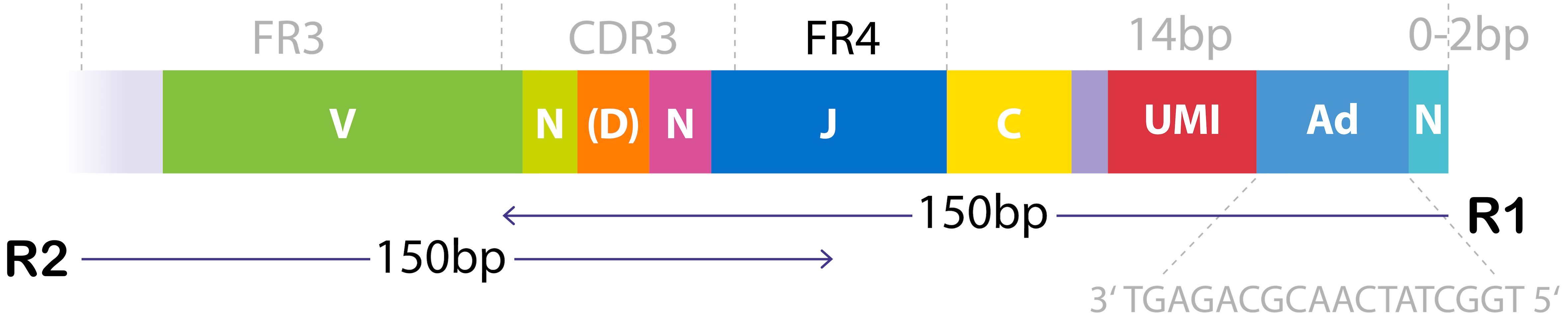
Figure 1. Structure of the TCR cDNA library used for paired-end sequencing.

The Miltenyi TCR Clonotyping Block in Platforma uses MiXCR with a preset tuned specifically to this kit chemistry. It automates alignment, UMI deduplication, clonotype assembly, and quality control, producing a standardized clonotype dataset ready for downstream analysis blocks.

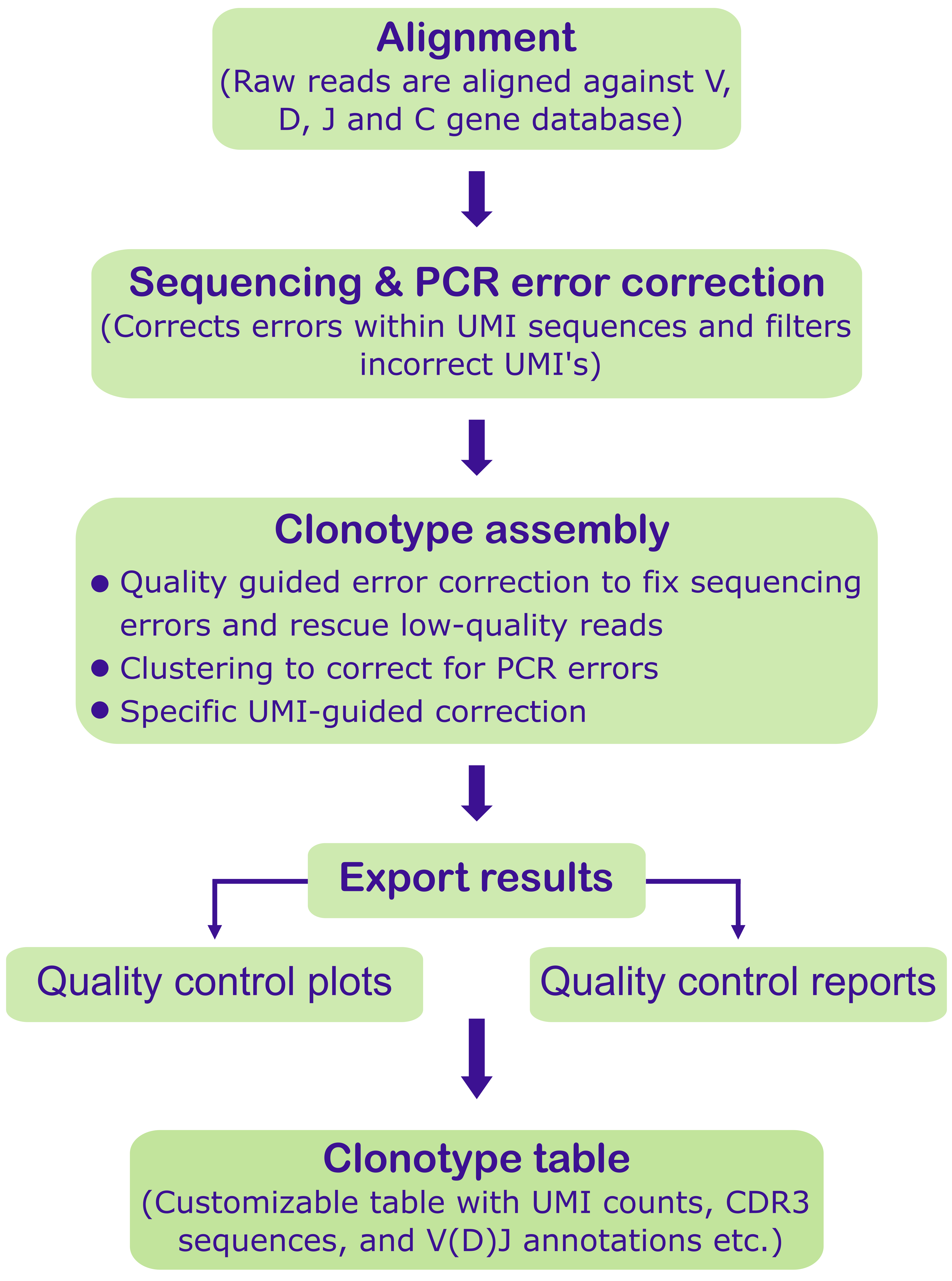
Figure 2. Overview of data processing steps performed by the Miltenyi TCR Clonotyping block.

note

When using this block in your research, please cite the MiXCR publication:

Bolotin, D. A., Poslavsky, S., Mitrophanov, I., Shugay, M., Mamedov, I. Z., Putintseva, E. V., & Chudakov, D. M. (2015). MiXCR: software for comprehensive adaptive immunity profiling. Nature Methods, 12(5), 380–381. https://doi.org/10.1038/nmeth.3364

---

Tutorial dataset

The example data comes from a 43-year-old healthy male donor followed over approximately two years. The donor received a SARS-CoV-2 vaccine in January 2021 and subsequently experienced two infections: a sequencing-confirmed Alpha variant infection (April 2021) and a likely Omicron infection (January 2022). PBMCs were collected at 10 time points with two replicates each. TCRβ chains were sequenced on an Illumina platform (150 × 150 bp paired-end reads).

Figure 3. Sample collection timeline showing vaccination, Alpha infection (T3), and Omicron infection (T8).

The dataset originates from Discovery of rare antigen-specific TCRs via replicate profiling (https://doi.org/10.1101/2025.09.30.675572) and is publicly available under ENA accession PRJNA995237.

tip

This dataset includes TCRβ only, matching the published study, as the highly diverse CDR3 region of the β chain contributes the most to epitope recognition. The Miltenyi TCR Clonotyping Block supports both TCRα and TCRβ — you can run both chains simultaneously on your own data by selecting both in the block settings.

---

Before you start

• Platforma desktop app — install the latest version (see Installation).
• Input files — paired-end FASTQ files produced with Miltenyi Biotec's TCR α/β RNA Profiling Kit, human (catalog no. 130-139-385). See How to Import Data for a detailed import walkthrough.
• Sample metadata (optional but recommended) — a TSV or Excel file with at least one column identifying each sample's condition or time point. Download the metadata file used in this tutorial.

---

---

Setting up the analysis

Create a new project

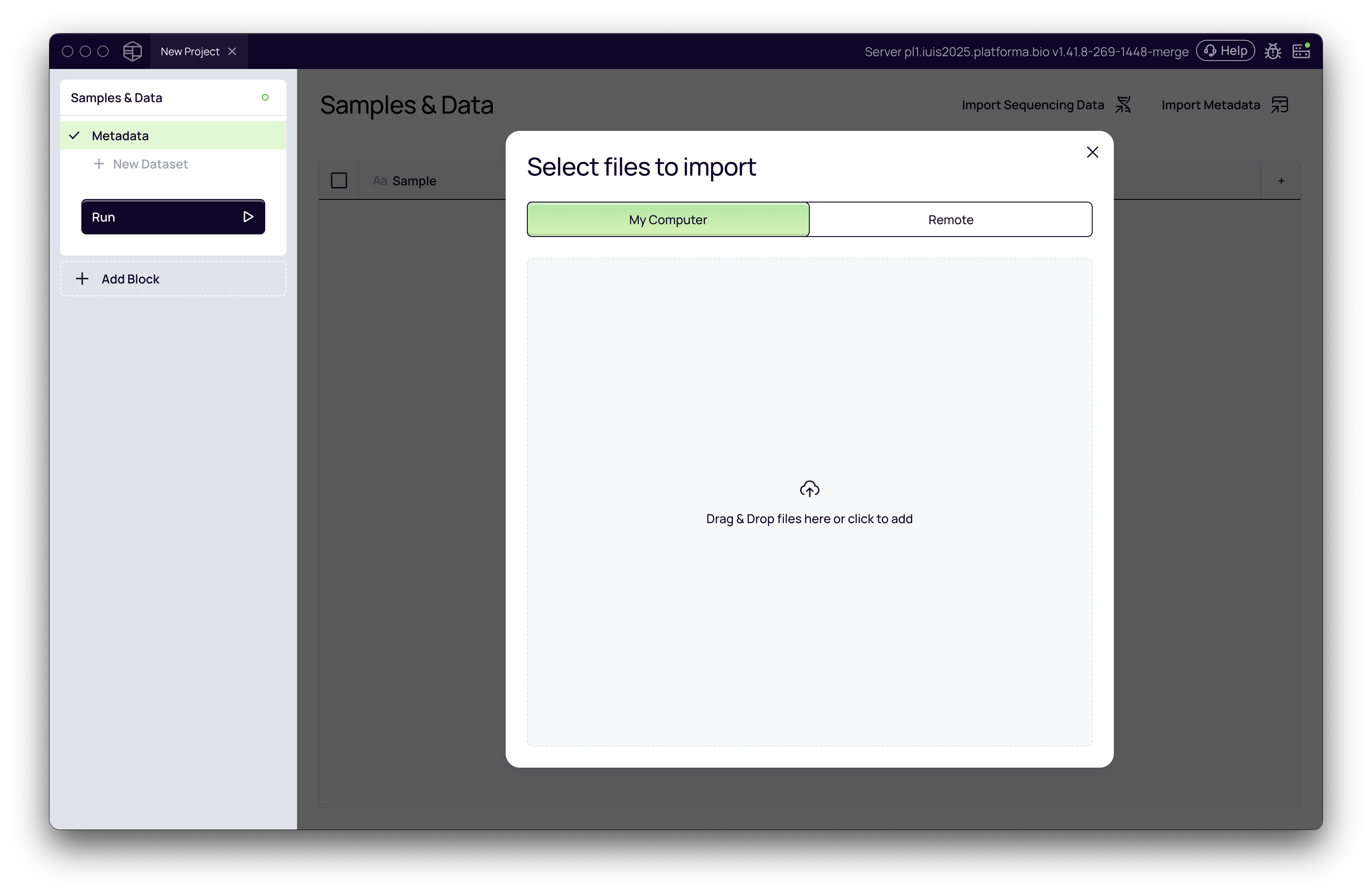
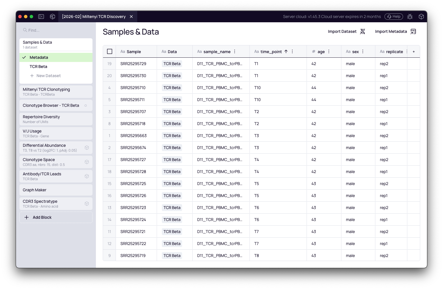
Open Platforma and create a new project. The Samples & Data block is added automatically — this is where you will import your files.

Import FASTQ files

1. In the Samples & Data block, click Add data and choose your source (local files or remote storage).
2. Select all paired-end FASTQ files for your experiment.
3. Platforma automatically detects sample names and pairs R1/R2 reads from the filenames. Adjust the filename pattern if needed.
4. Give the dataset a name (e.g., Miltenyi-TCR-Beta) and click Create Dataset.

note

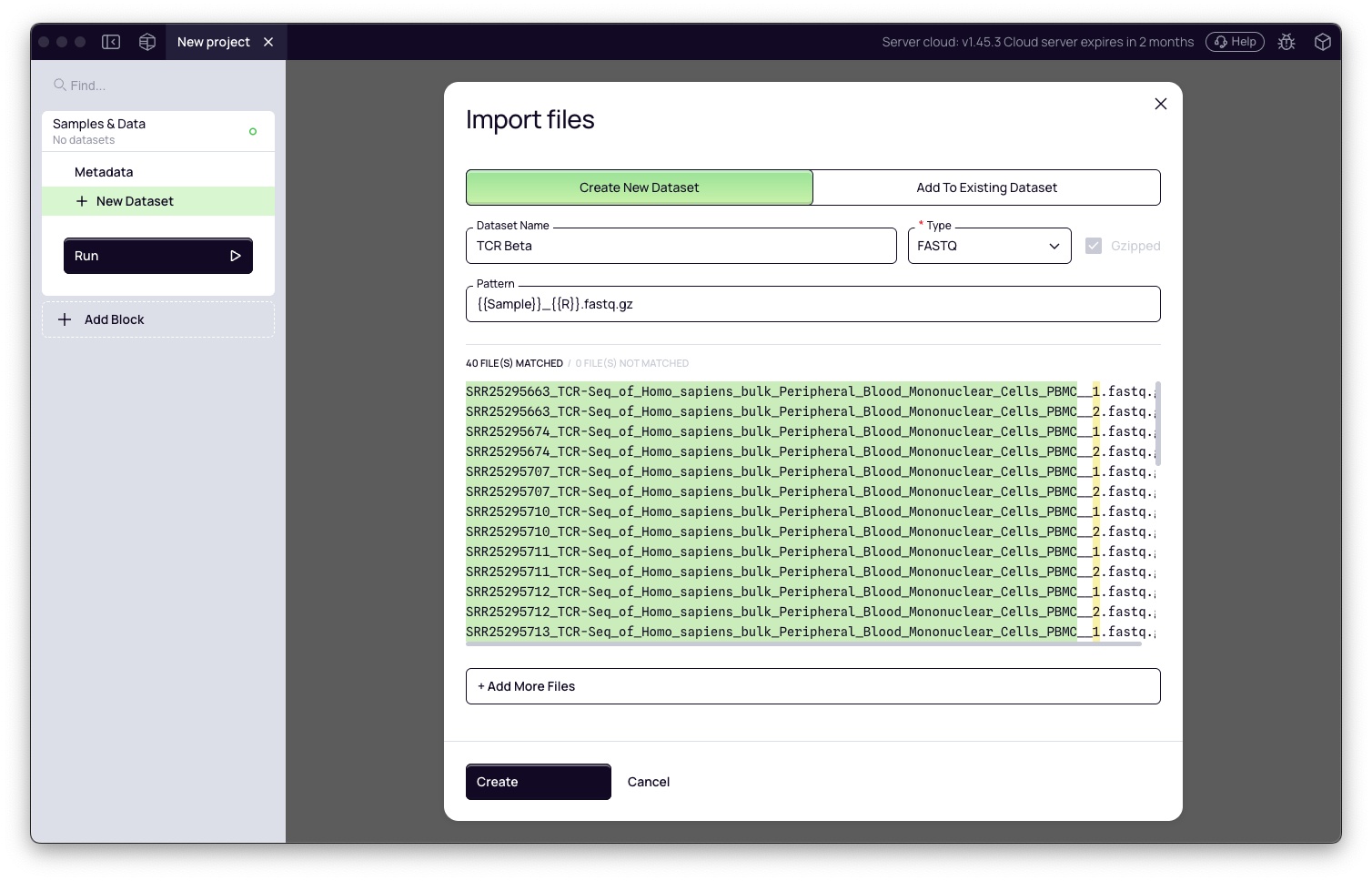
For this tutorial, download the 40 FASTQ files (10 time points × 2 replicates × 2 reads per replicate) from ENA accession PRJNA995237. Select only the bulk PBMC files. Example filename for time point 1, replicate 1:

D11_PBMC_PBMCtp01_1_TRB_S90_R1_001.fastq.gz

Depending on how you download from ENA, files may also appear with SRR-prefixed names (e.g., SRR25295730_1.fastq.gz / SRR25295730_2.fastq.gz). Platforma will auto-pair R1/R2 files regardless of naming convention.

Import sample metadata

1. In the Samples & Data block, click Add metadata.
2. Select your Excel or TSV sample sheet.
3. Map the time point (or condition) column so Platforma can use it for grouping in downstream analyses.

Configure the Miltenyi TCR Clonotyping block

1. Click + Add Block in the left-hand panel.
2. Find and select Miltenyi TCR Clonotyping from the catalog.

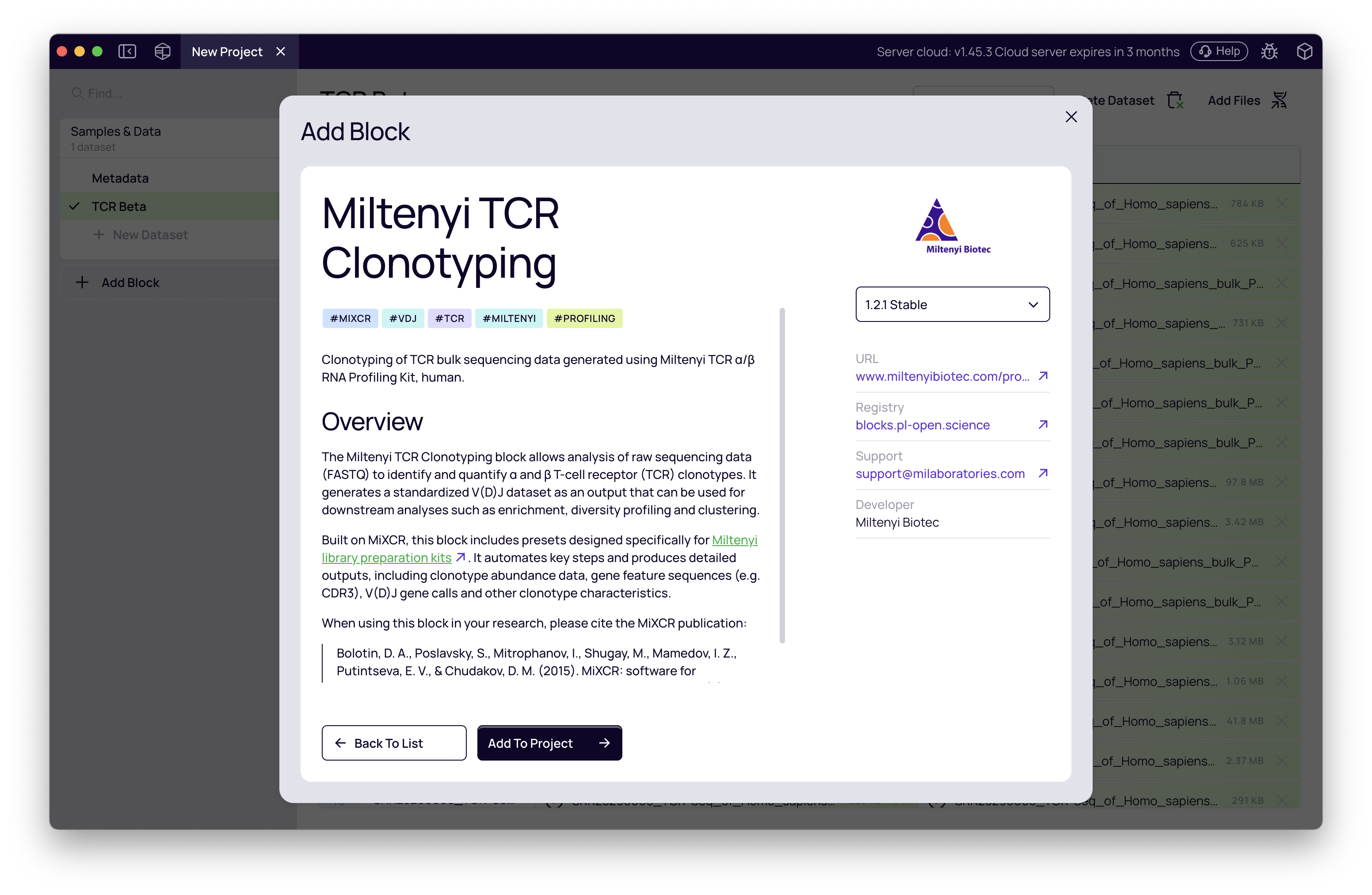
3. In the block settings panel on the right, configure the following:

Setting	Value for this tutorial	Notes
Input dataset	Miltenyi-TCR-Beta	The FASTQ dataset created above
Preset	TCR α/β RNA Profiling Kit, human	Default — tuned for this kit
Chains	TCR beta	Tutorial uses TCR beta only; select both TCR alpha and TCR beta for α+β experiments

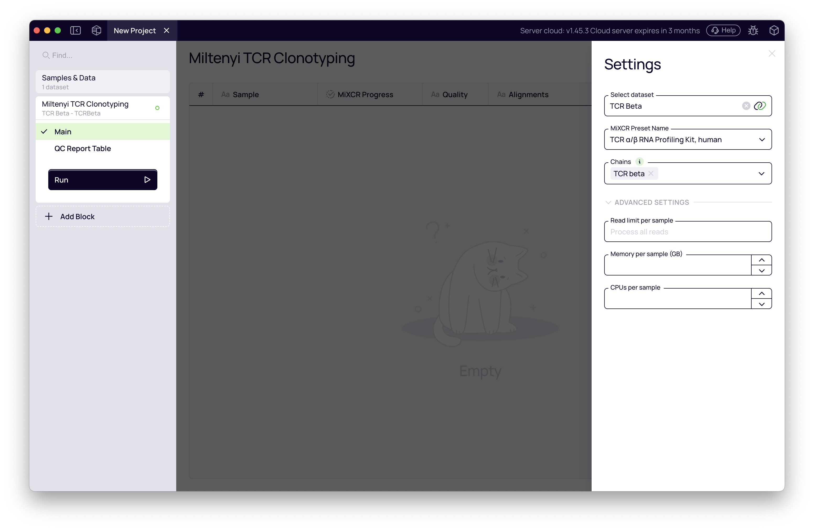
4. Click Run.

tip

For a quick validation before running all 20 samples, enable Limit reads under Advanced Settings (e.g., 10,000 reads per sample). The run completes in minutes and lets you verify the pipeline before committing to the full analysis.

---

Quality control

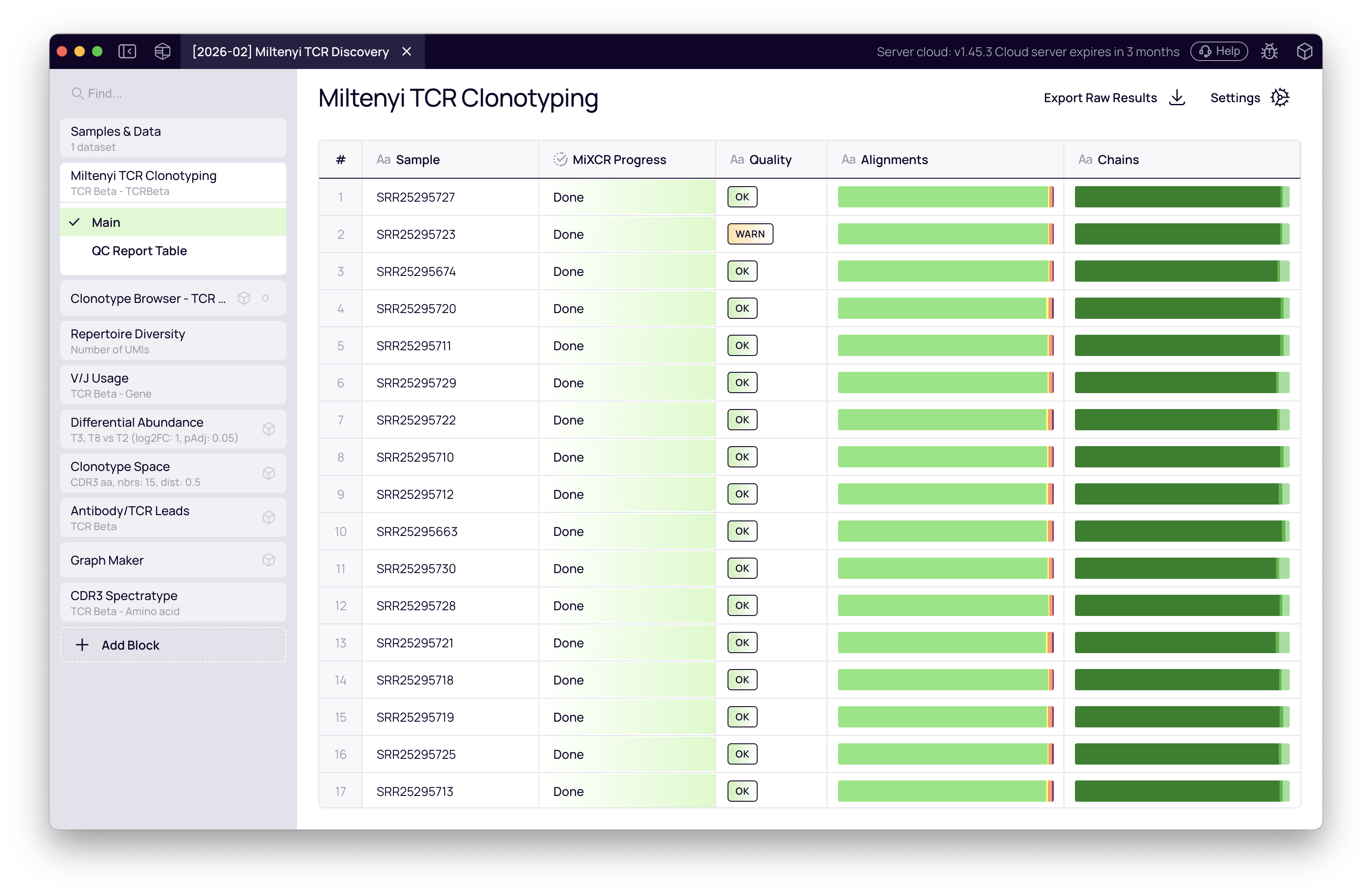
QC overview table

When the run completes, the block displays a QC overview table with one row per sample. Key columns:

• Quality — flags WARN or ALERT if any check is triggered.
• Alignment — stacked bar showing aligned vs. non-aligned reads. For targeted multiplex libraries, expect >85% alignment.
• Chains — proportion of reads assigned to each chain.

All 20 samples passing with high alignment rates and no alerts indicates the run is clean and ready for downstream analysis.

Per-sample detail

Click any sample to open its detailed QC report.

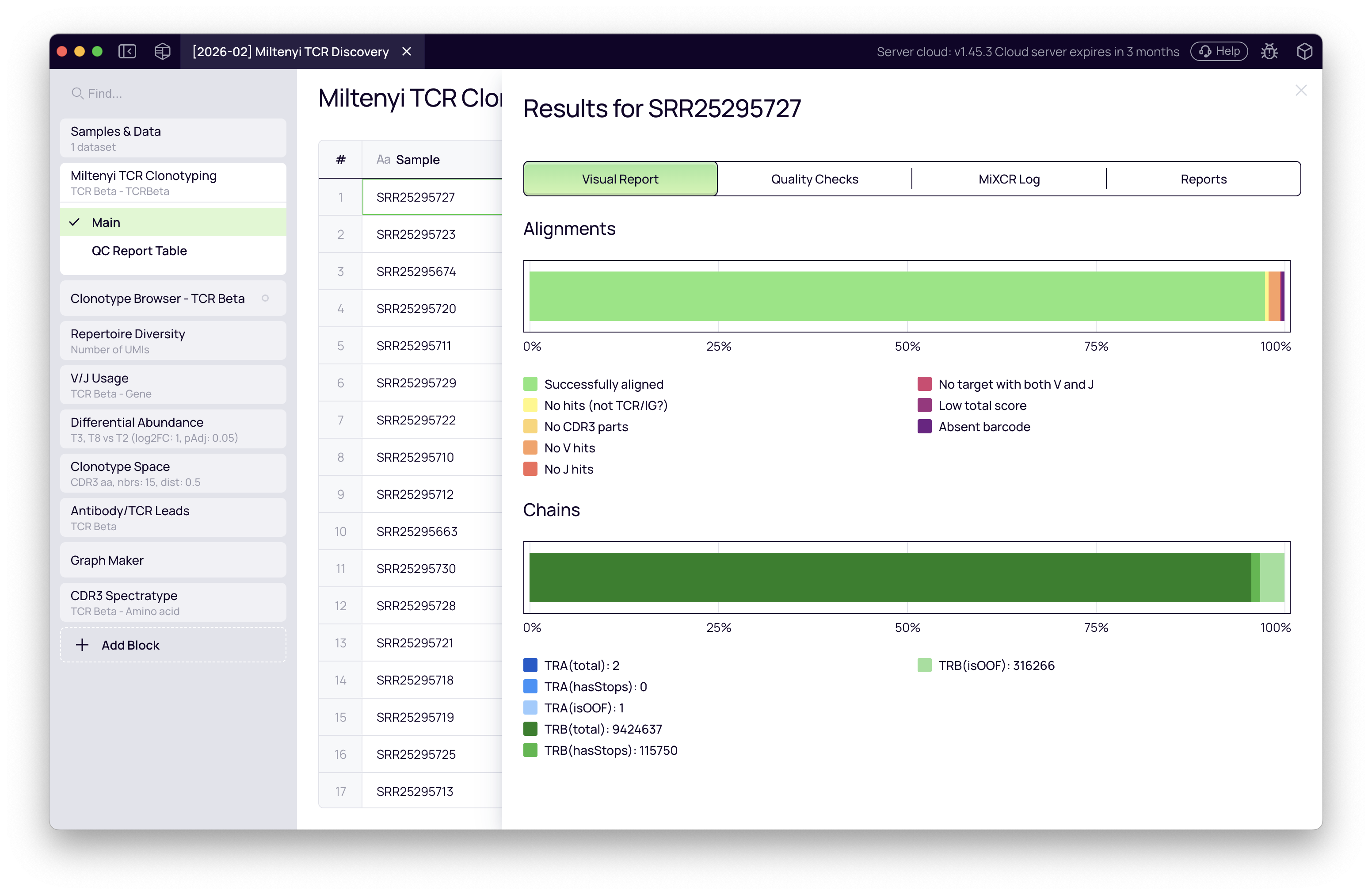
The Quality Checks tab lists every metric MiXCR evaluated. A sample from the tutorial dataset may trigger a warning on reads used in clonotypes if sequencing depth differs across replicates — this is expected and visible in the rarefaction analysis later. The Log tab provides the full MiXCR report for troubleshooting.

For the full list of QC metrics and their interpretation, see the MiXCR QC documentation.

---

Clonotype output

The block produces a clonotype table for each chain analyzed. For this tutorial that is one TCR beta table with 20 columns (one per sample). Each row is a unique clonotype characterized by:

• Abundance — UMI count and fraction per sample
• CDR3 — amino acid and nucleotide sequences
• V/J gene calls — best-match gene assignments

The raw clonotype tables are exportable as TSV files directly from the block. To browse clonotypes interactively, add a Clonotype Browser block — it connects to the clonotyping output automatically and lets you inspect per-sample clonotype lists and cross-sample overlaps.

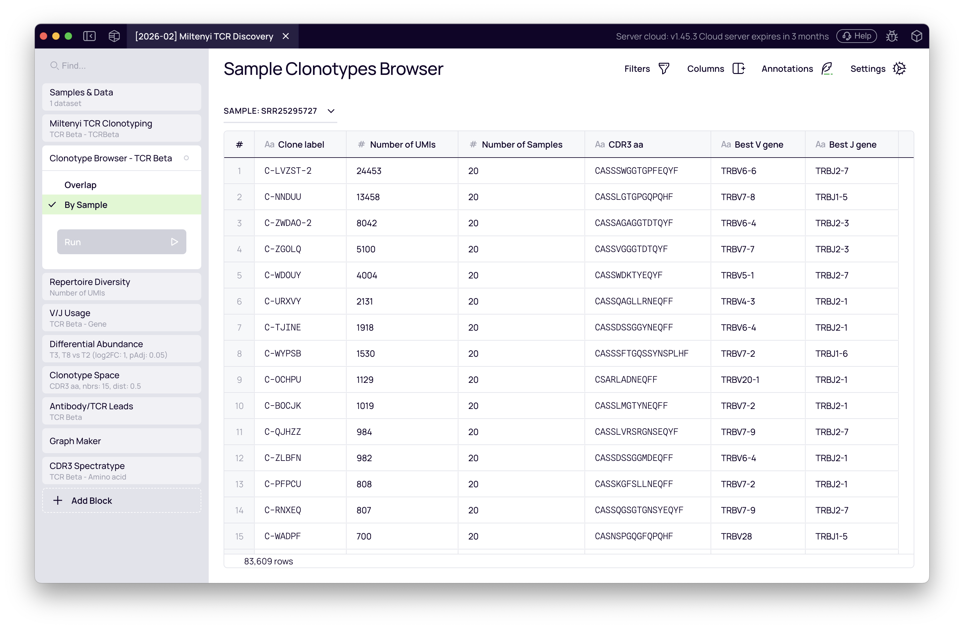
This standardized output is also what all downstream analysis blocks query automatically — no manual connection is needed.

---

Diversity and clonality analysis

Question: Is there a clonal expansion at the infection time points?

1. Click + Add Block and add the Diversity Analysis block.
2. It automatically connects to the clonotyping output.
3. In the settings, group samples by the time point column from your metadata.

The block computes per-sample diversity metrics including Chao1 richness estimate, clonality, and dominance. Switch the view to line plot to see how metrics evolve across time points.

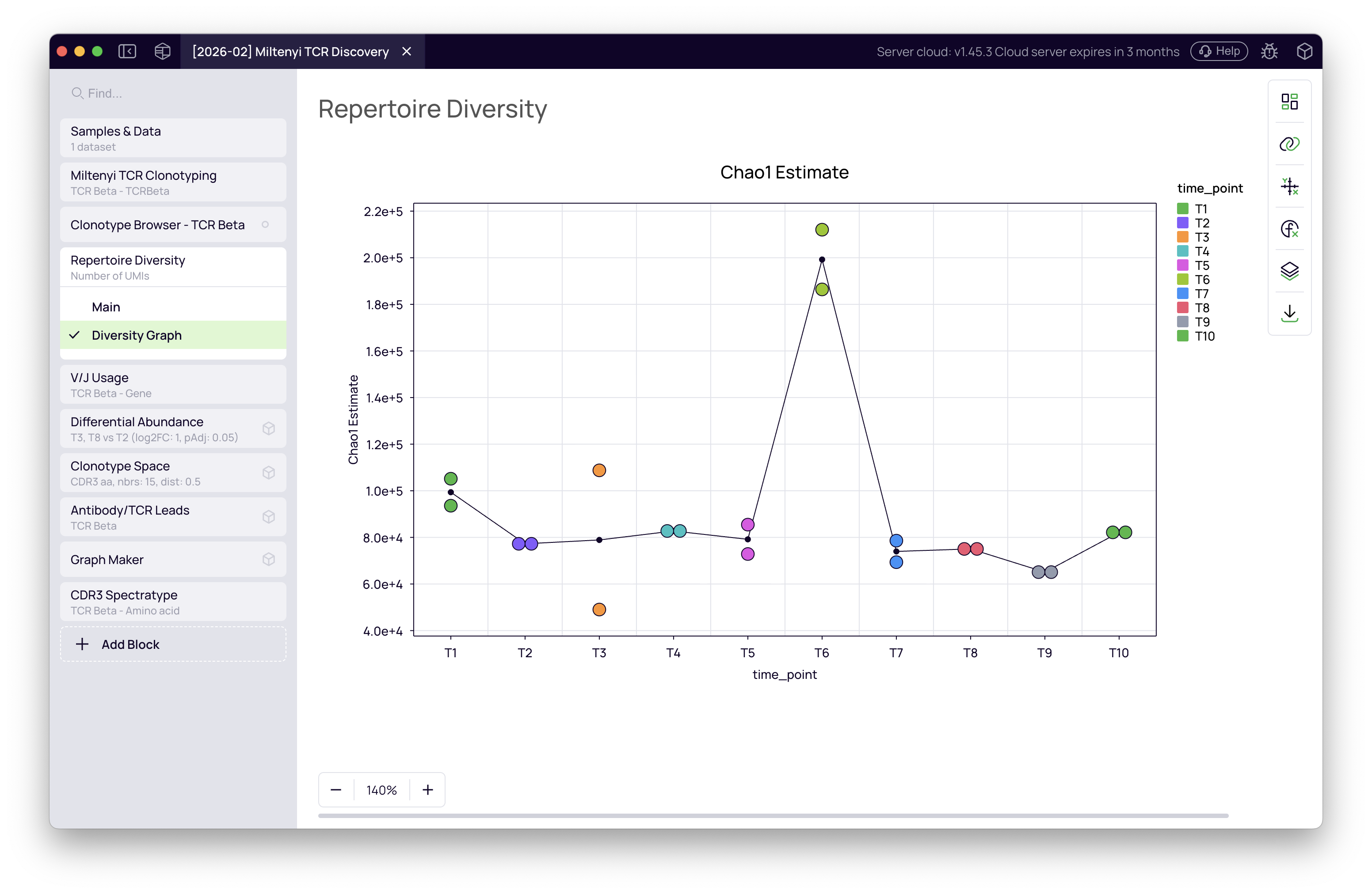
T6 stands out with a notably higher diversity estimate. This is a sequencing depth artefact — T6 samples were sequenced more deeply than the others, so the Chao1 estimator projects a higher theoretical richness. It is not a biological signal. The infection-driven clonal expansions will become visible in the differential abundance analysis below.

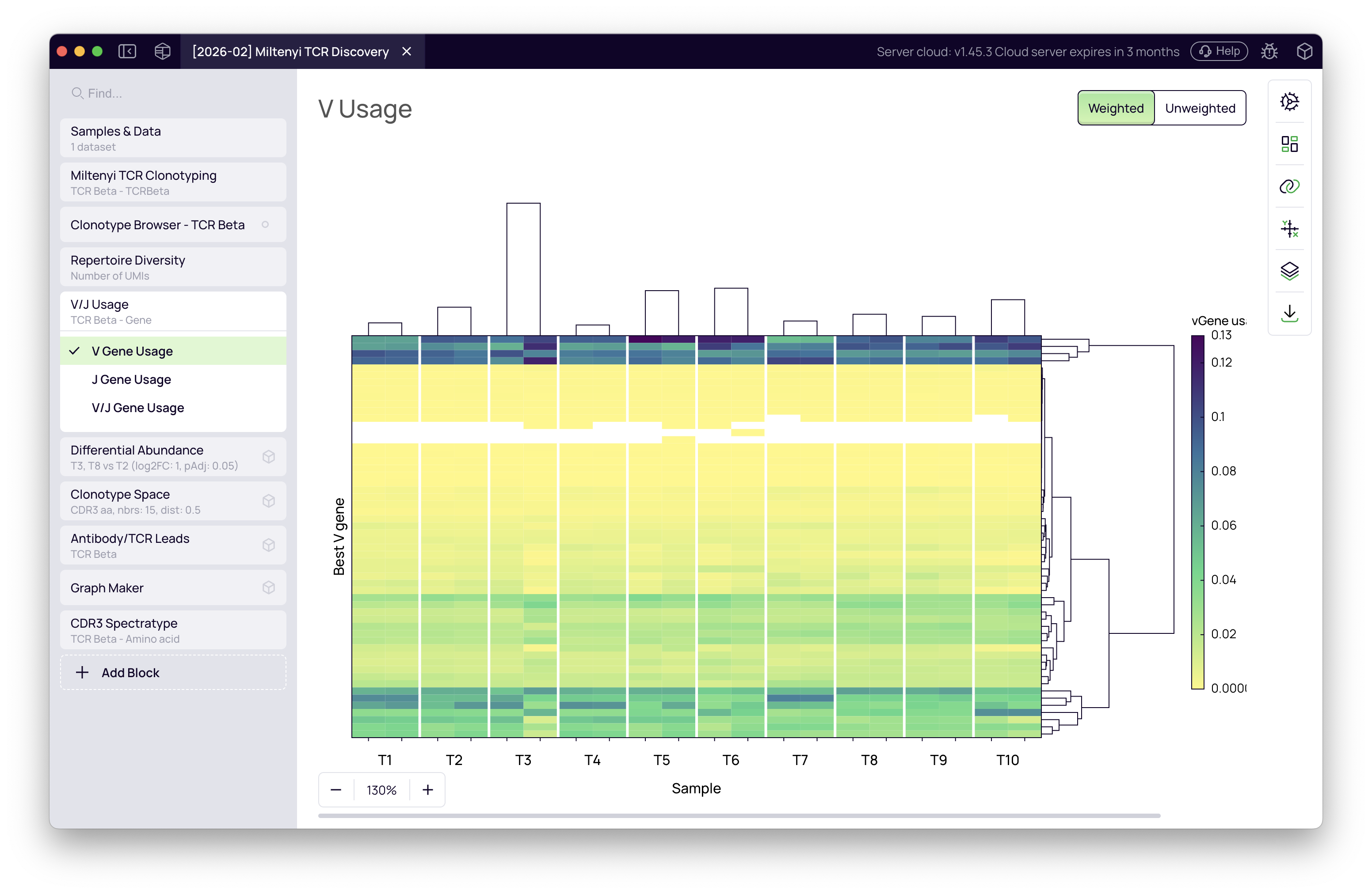
Gene usage:

The block also shows V and J gene distribution across samples. Expand the Gene Usage tab to visualize whether certain gene segments are enriched at specific time points.

---

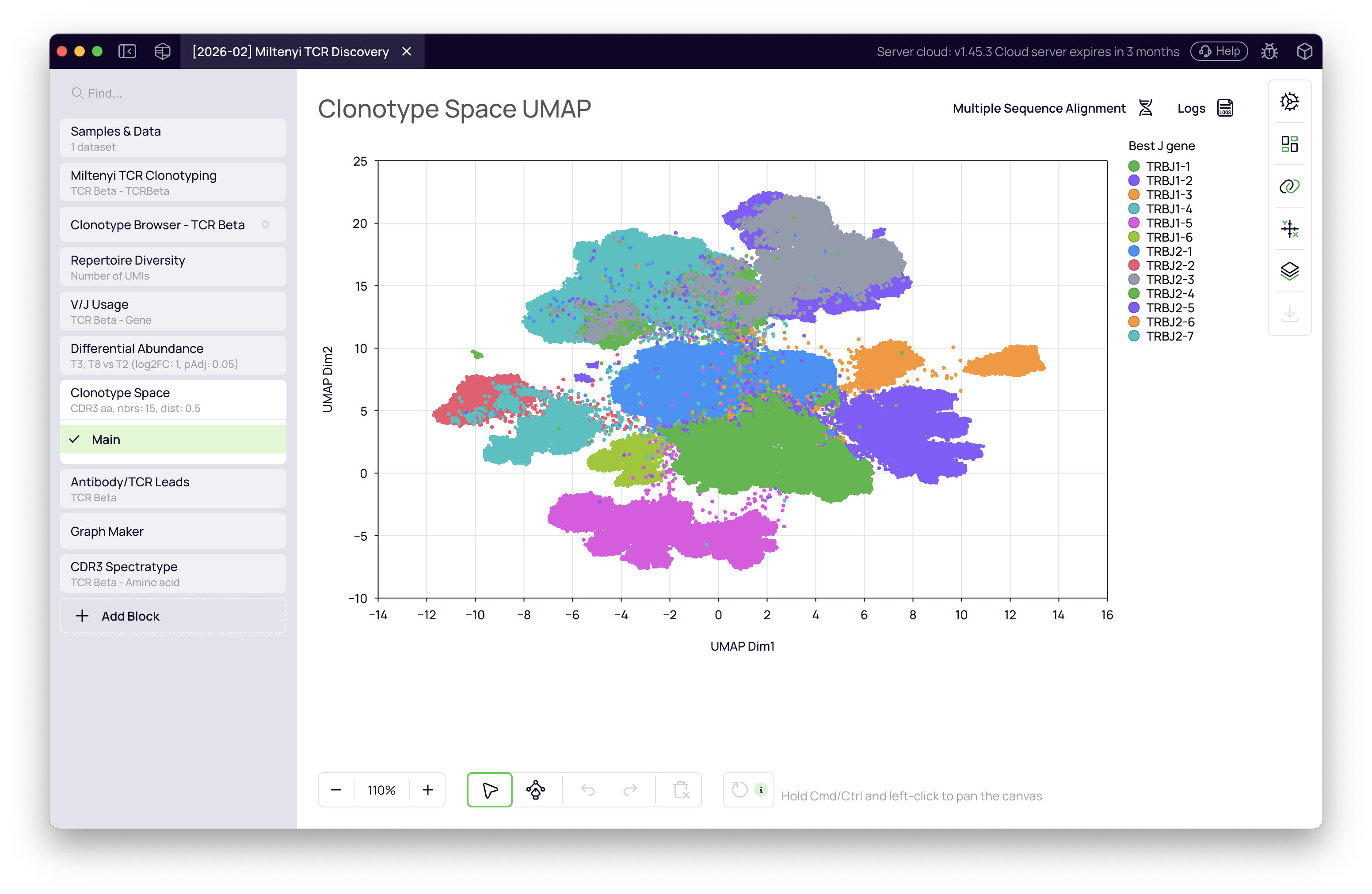
Clonotype Space

Question: What does the full TCR landscape look like?

1. Add the Clonotype Space block.
2. It connects to the clonotyping output automatically.

The block embeds all clonotypes in a UMAP where proximity reflects sequence similarity. Each dot represents one clonotype; dot size encodes abundance. Color the map by J gene to reveal structural organization — J gene families cluster spatially across the repertoire.

---

Differential abundance

Question: Which clonotypes are specifically activated by the COVID infections?

T2 is the last time point before the first infection — post-vaccine but pre-COVID. Comparing T3 and T8 against T2 isolates clones activated specifically by infection rather than by vaccination.

1. Add the Differential Abundance block.
2. It connects to the clonotyping output automatically.
3. Configure two comparisons using the time point metadata column:
   • T3 vs T2 — clones activated by the Alpha infection
   • T8 vs T2 — clones activated by the Omicron infection

The block displays a volcano plot for each comparison — log2 fold change on the X-axis, significance on the Y-axis. Clonotypes in the upper-right quadrant are significantly expanded in the test group.

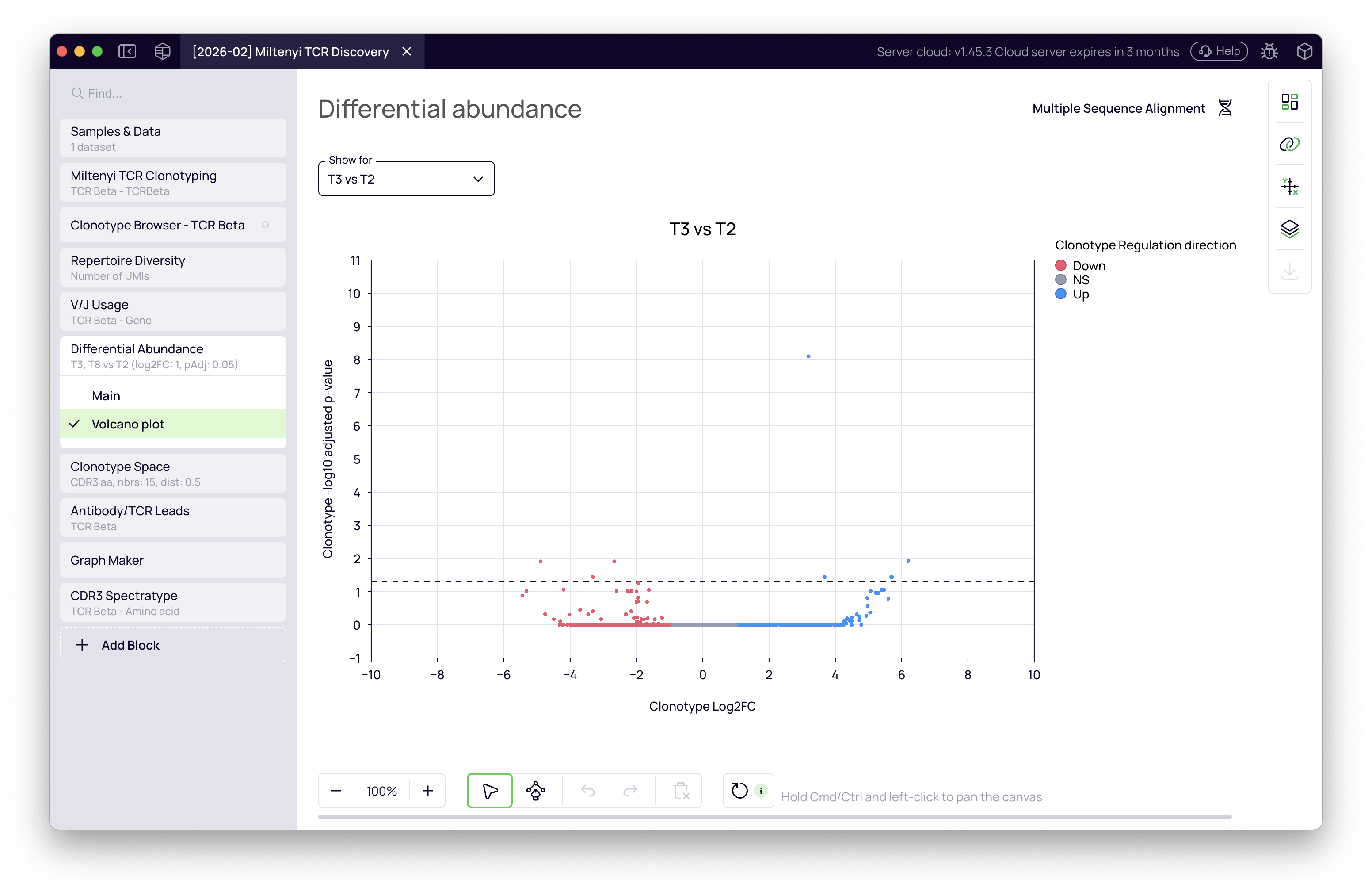
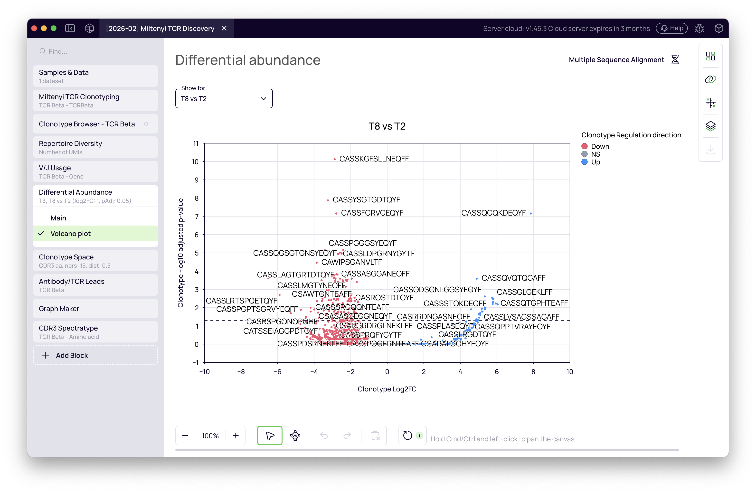
The T8 vs T2 comparison shows a stronger signal, consistent with the more severe Omicron infection this donor experienced. The upregulated clonotype list from this comparison is what we carry into the next steps.

---

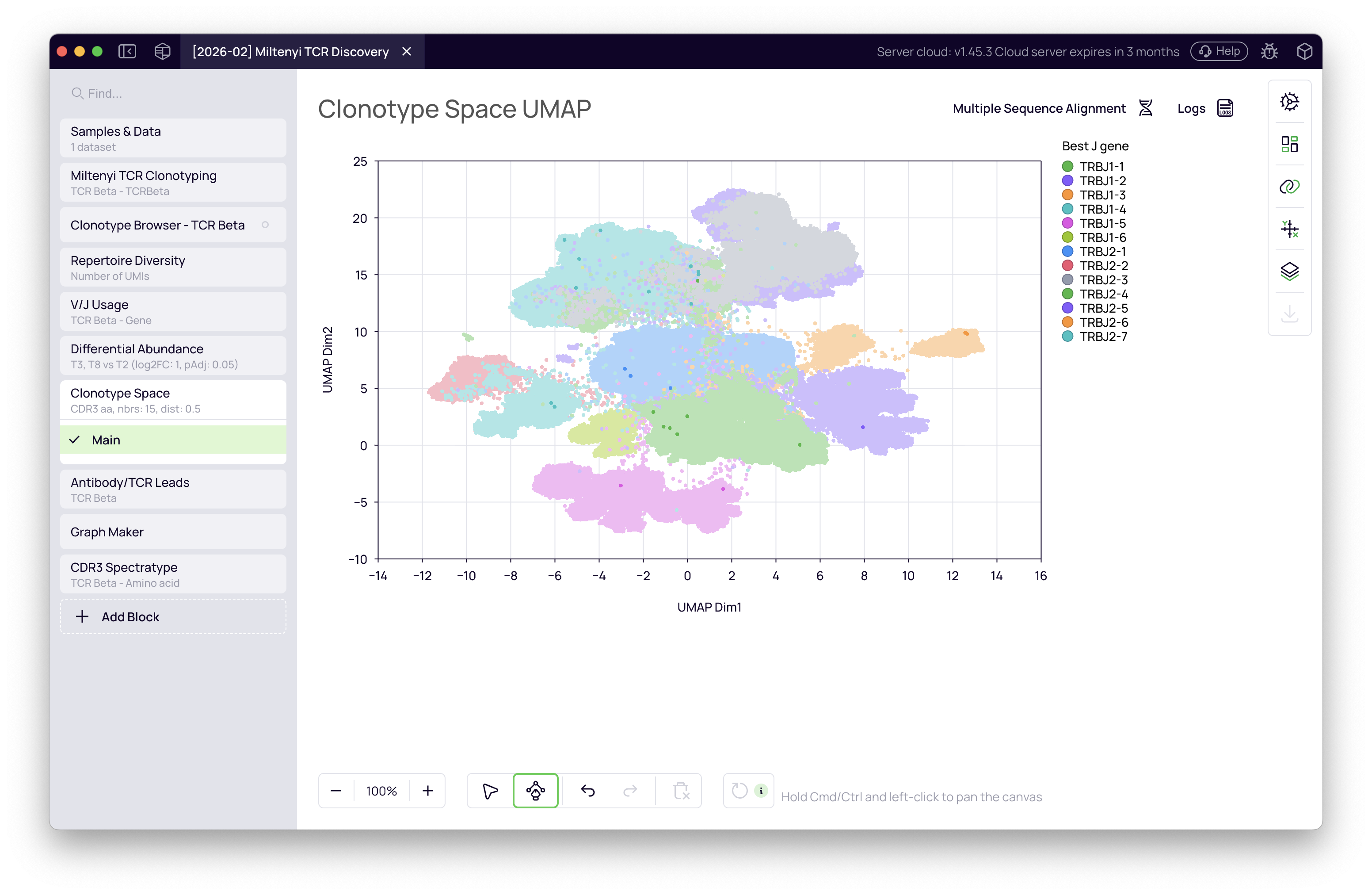
Clonotype Space — infection-expanded clones in context

With the T8 vs T2 upregulated clonotypes identified, return to the Clonotype Space and overlay the differential abundance result. The upregulated clonotypes are highlighted on the UMAP, revealing where the infection-expanded T cells sit within the full repertoire landscape.

---

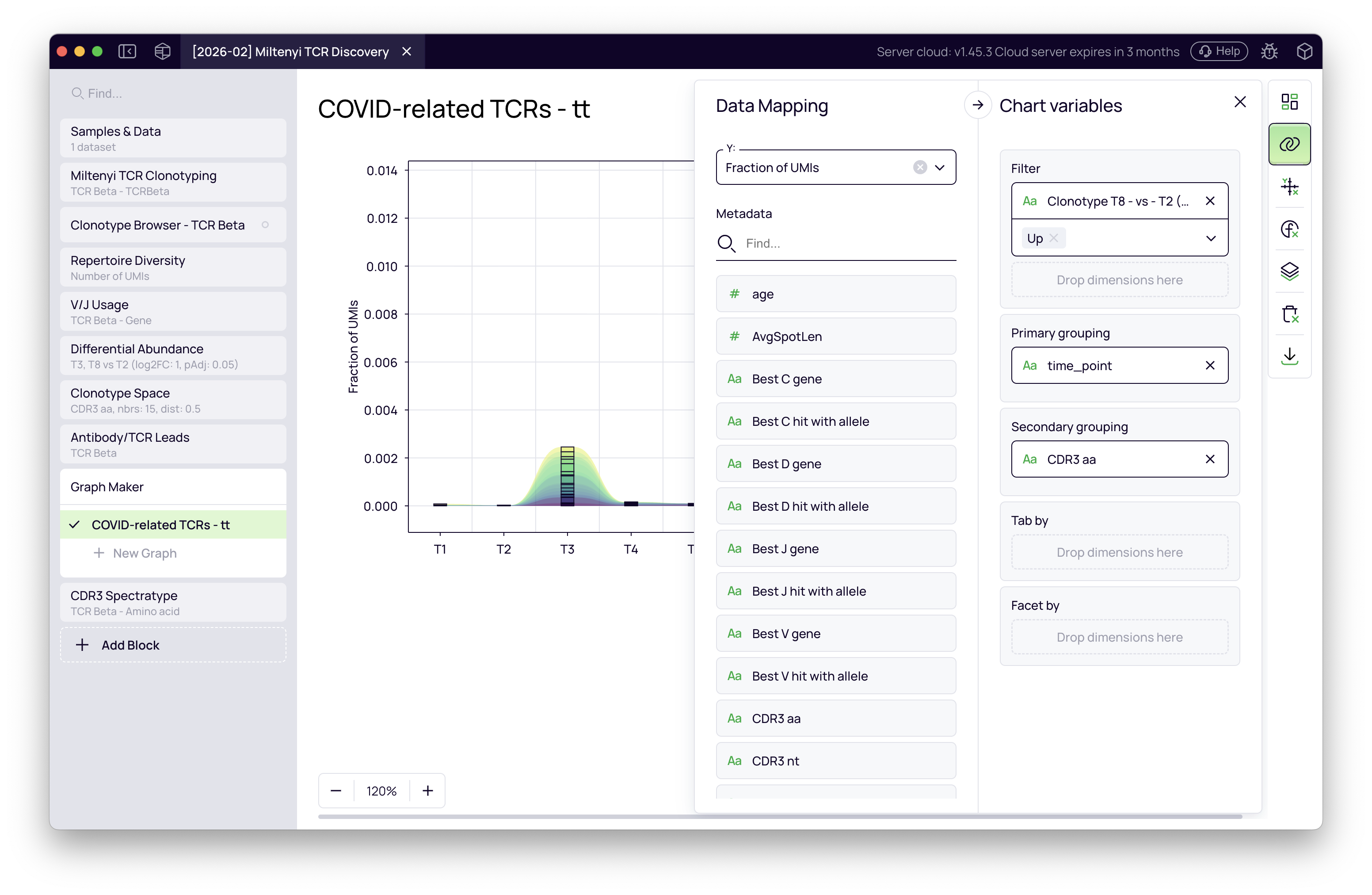
Clone tracking with Graph Maker

Question: How do the infection-expanded clones behave across the full 1.5-year timeline?

1. Add the Graph Maker block.
2. Configure the plot:
   • Plot type — Stream area (or stacked bar)
   • X-axis — time point
   • Y-axis — clonotype fraction (UMI-normalized abundance)
   • Filter — clonotypes upregulated in the T8 vs T2 differential abundance result
   • Color — CDR3 amino acid sequence (one color per unique clone)

The resulting figure tracks each COVID-associated clone individually across all 10 time points. The clones expand at T8 (Omicron) and — strikingly — show a smaller but clear activation at T3 (Alpha) as well, even though the comparison was designed around T8. This cross-reactivity emerges directly from the data without any additional filtering.

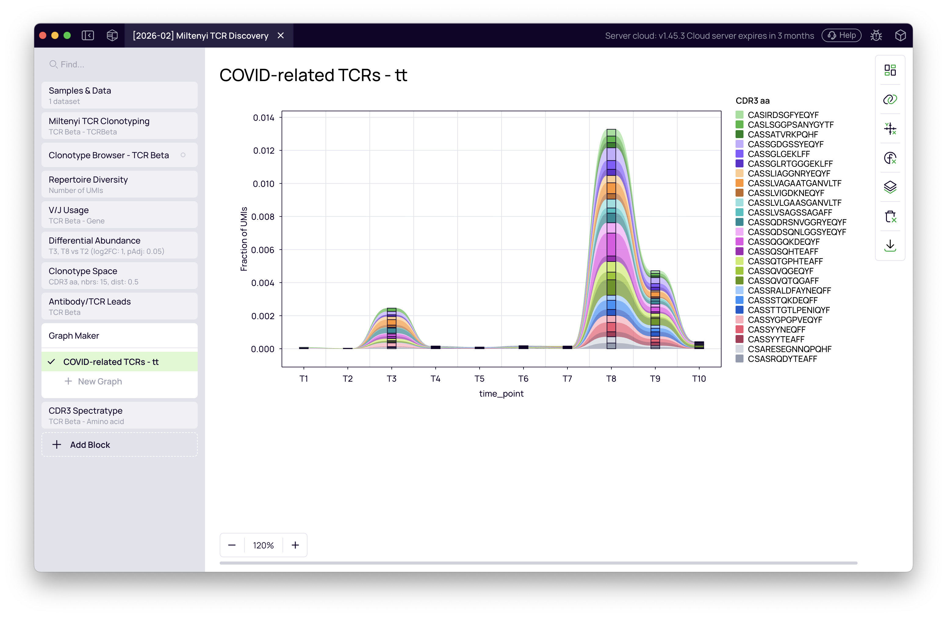
This figure is directly exportable for publication.

---

Summary

Starting from 20 paired-end FASTQ files, this tutorial covered:

1. Clonotyping — FASTQ → verified clonotype table with UMI-normalized abundance, CDR3 sequences, and V/J gene calls
2. Diversity analysis — repertoire-wide metrics across time; T6 elevation explained as a sequencing depth artefact
3. Clonotype Space — full TCR landscape visualized by J gene
4. Differential abundance — T3 vs T2 and T8 vs T2 comparisons identify infection-specific clones; T8 signal highlighted back onto the UMAP
5. Clone tracking — COVID-associated clones tracked across 1.5 years; cross-reactivity between Alpha and Omicron visible in a single exportable figure

Total time from import to final figure: a few hours, no code.

Resources:

• Webinar: Streamlining TCR α/β discovery — Miltenyi Biotec & MiLaboratories
• Miltenyi TCR α/β RNA Profiling Kit, human
• Tutorial dataset — ENA PRJNA995237
• MiXCR documentation